
Graphical Method of LPP: Steps, Solved Example and Corner Point Method
Публикувано на October 16, 2026 · от Simplex Method Calculator Editorial Team
The graphical method is the most visual way to solve a linear programming problem (LPP). It works only for problems with two decision variables, because you need to draw them on an x1–x2 plane, but it shows clearly what every LP solution method is really doing: searching the corners of a feasible region for the best value of the objective.
This guide gives the steps, solves one complete example with a graph, and shows how the same answer comes out of the simplex method.
Graphical Method Steps
- Write the LPP with the objective and every constraint, including x1, x2 ≥ 0.
- Draw each constraint as a line. Replace the inequality with an equals sign and find the two intercepts (set x1 = 0, then x2 = 0).
- Shade the correct side of each line. Test the origin (0, 0): if it satisfies a ≤ constraint, shade towards the origin; otherwise shade away from it.
- Find the feasible region, the area that satisfies every constraint at the same time.
- Find the corner points of the feasible region, either by reading intercepts or by solving pairs of line equations.
- Evaluate the objective at every corner. The best value is the optimum. This is called the corner point method.
The rule behind step 6 is the fundamental theorem of linear programming: if an LP has an optimal solution, at least one optimal solution lies at a corner point of the feasible region.
Solved Example
A furniture maker produces chairs (x1) and tables (x2). Each chair earns 50 and each table earns 40.
- Maximize Z = 50x1 + 40x2
- Subject to 3x1 + 5x2 ≤ 150 (assembly hours)
- x2 ≤ 20 (table demand)
- 8x1 + 5x2 ≤ 300 (wood)
- x1, x2 ≥ 0
Step 1: Draw the Constraint Lines
| Constraint | Line | Intercept on x1 axis | Intercept on x2 axis |
|---|---|---|---|
| Assembly | 3x1 + 5x2 = 150 | (50, 0) | (0, 30) |
| Table demand | x2 = 20 | none (horizontal line) | (0, 20) |
| Wood | 8x1 + 5x2 = 300 | (37.5, 0) | (0, 60) |
The origin satisfies all three ≤ constraints (0 ≤ 150, 0 ≤ 20, 0 ≤ 300), so each region lies on the origin’s side of its line.
Step 2: Find the Feasible Region and Its Corners
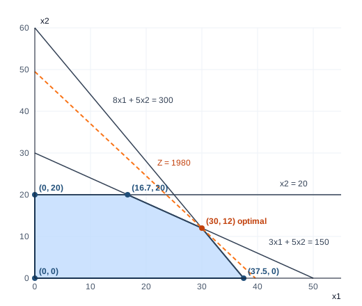
The shaded area in the graph is the feasible region. It has five corners:
- (0, 0), the origin
- (37.5, 0), where the wood line meets the x1 axis
- (0, 20), where the demand line meets the x2 axis
- (16.7, 20), where the assembly line meets x2 = 20: 3x1 + 5(20) = 150 gives x1 = 50/3 ≈ 16.67
- (30, 12), where the assembly and wood lines cross
The last corner needs a small system of equations. Subtract 3x1 + 5x2 = 150 from 8x1 + 5x2 = 300 to get 5x1 = 150, so x1 = 30. Then 3(30) + 5x2 = 150 gives x2 = 12.
Step 3: Evaluate the Objective at Each Corner
| Corner (x1, x2) | Z = 50x1 + 40x2 |
|---|---|
| (0, 0) | 0 |
| (37.5, 0) | 1,875 |
| (0, 20) | 800 |
| (16.67, 20) | 1,633.33 |
| (30, 12) | 1,980 |
Answer
The maximum profit is Z = 1,980 at x1 = 30 chairs and x2 = 12 tables. Check: assembly 3(30) + 5(12) = 150 ✓ (fully used), demand 12 ≤ 20 ✓ (8 tables of unused demand), wood 8(30) + 5(12) = 300 ✓ (fully used).
The Iso-Profit Line Method
Instead of testing every corner, you can draw the objective as a line, for example 50x1 + 40x2 = 1,000, and slide it parallel to itself away from the origin. The last point of the feasible region it touches is the optimum. In the graph, the dashed orange line is the iso-profit line at its final position, Z = 1,980, touching the region only at (30, 12). For minimization problems, slide the line towards the origin instead.
Special Cases on a Graph
- Multiple optimal solutions: the objective line is parallel to an edge of the feasible region, so the whole edge is optimal.
- Unbounded solution: the feasible region is open in the direction that improves Z.
- Infeasible problem: the shaded regions have no common area.
- Redundant constraint: a line that does not touch the feasible region at all. Removing it does not change the answer.
The same four cases appear in tableau form in special cases in the simplex method.
Graphical Method vs Simplex Method
The simplex method follows the same corners, but algebraically. Solving this problem with the simplex method starts at (0, 0), moves to the corner (37.5, 0) and then to (30, 12), where the Cj − Zj row shows that no neighbouring corner is better. The graphical method checks all five corners; the simplex method visits only three. For more than two variables, drawing is impossible and the simplex method is the only practical option. A full comparison is in simplex method vs graphical method.
Common Mistakes
- Shading the wrong side of a ≥ constraint. Always test a point such as the origin.
- Missing a corner where two constraint lines cross inside the first quadrant.
- Reading coordinates off the graph by eye. Solve the two line equations to get exact values.
- Forgetting x1, x2 ≥ 0, which limits the region to the first quadrant.
Check Your Answer
Enter 50x1 + 40x2 and the three constraints in the 2-variable simplex calculator to confirm the optimum x1 = 30, x2 = 12, Z = 1,980 and to see the simplex tableaus that reach the same corner.